A video of the presentation (in French)) :

Goal
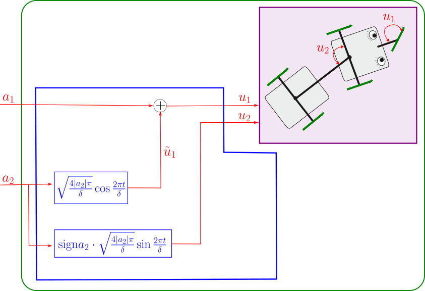
We show that skating or swimming corresponds more or less to a control based on Lie brackets.
For this purpose, we consider a snake like car, standing on five ice skates, which is designed to move on a frozen lake.
We propose to apply the lie brackets between the two input fields.
These brackets create a new direction in the state space that can now be controlled.
Another contribution of this works is to show that it is possible to move extremely fast along a direction created by Lie brackets.
Code for the simulation of the snake robot
The following simulation illustrates how Lie brackets can be used for propulsion.
The vehicle is a snake like car, standing on five ice skates.
from roblib import *

def f(x,u):
    mx,my,θ,v,α,β=list(x[0:6,0])
    u1,u2=list(u[0:2,0])
    return array([[v*cos(θ)],[v*sin(θ)],[v*β],[-(β+sin(α))*u2],[-v*(β+sin(α))],[u1]])

def draw_snake(x):
   mx,my,θ,v,α,β=list(x[0:6,0])
   M0=array([[ 0  ,-0.3, 0.3, 0  ,0  ,-0.3,0.3,0  ,0,1],
             [-0.4,-0.4,-0.4,-0.4,0.4, 0.4,0.4,0.4,0,0]])
   M0=add1(M0)
   W=array([[-0.4,0.4],[0,0],[1,1]])
   R1=tran2H(mx,my)@rot2H(θ)
   M1=R1@M0
   skate=R1@tran2H(1,0)@rot2H(arctan(β))@W
   M2=R1@rot2H(α)@tran2H(-1,0)@M0
   plot2D(M1,'blue',1)
   plot2D(skate,'magenta',1)
   plot2D(M2,'black',1)


def liesnake():
    ax = init_figure(-2,35,-2,0.6*35)
    tmax,deltak=0.9,50
    x=array([[0],[0],[2],[0.1],[0],[0]]) #x,y,θ,v,α,β
    rLie=10 #Lie ratio
    dt=0.001
    δ=sqrt(dt)
    θbar=pi/6
    βbar=0
    vbar=100

    for t in arange(0,tmax,dt):
        clear(ax)
        draw_snake(x)
        def control_u_circle(a):
            a1,a2=list(a[0:2,0])
            eps= sign(a2)
            u = array([[cos(eps*2*pi*t/δ)],[sin(eps*2*pi*t/δ)]])
            A=δ*δ/3.14
            u=sqrt(4*abs(a2)*δ/A)*u+array([[a1],[0]])
            return u

        invA=array([[0,1],[-1,0]])
        mx,my,θ,v,α,β=list(x[0:6,0])
        βbar=0.95*βbar-0.03*sawtooth(θ-θbar)
        a=invA@(array([[5*(vbar-v)],[15*(βbar-β)]]))
        u=control_u_circle(a)
        _T.append(t)
        V.append(v)
        U1.append(u[0,0]*100)
        U2.append(u[1,0])
        x=x+dt*f(x+(dt/2)*f(x,u),u)
        pause(0.01)

V,_T,U1,U2=[],[],[],[]

if __name__ == "__main__":
    liesnake()
    figure()
    plot(_T,U1,"red")
    plot(_T,U2,"green")
    figure()
    plot(_T,V,"red")


